UPDATE: Compiled evaluation is now implemented for scikit-learn regression tree/ensemble models, available at https://github.com/ajtulloch/sklearn-compiledtrees or pip install sklearn-compiledtrees.

Our previous article on decision trees dealt with techniques to speed up the training process, though often the performance-critical component of the machine learning pipeline is the prediction side. Training takes place offline, whereas predictions are often in the hot path - consider ranking documents in response to a user query a-la Google, Bing, etc. Many candidate documents need to be scored as quickly as possible, and the top k results returned to the user.

Here, we'll focus on on a few methods to improve the performance of evaluating an ensemble of decision trees - encompassing random forests, gradient boosted decision trees, AdaBoost, etc.

There are three methods we'll focus on here:

• Recursive tree walking (naive)
• Flattening the decision tree (flattened)
• Compiling the tree to machine code (compiled)

We'll show that choosing the right strategy can improve evaluation time by more than 2x - which can be a very significant performance improvement indeed.

All code (implementation, drivers, analysis scripts) are available on GitHub at the decisiontrees-performance repository.

Naive Method

Superficially, decision tree evaluation is fairly simple - given a feature vector, recursively walk down the tree, using the given feature vector to choose whether to proceed down the left branch or the right branch at each point. When we reach a leaf, we just return the value at the leaf.

In Haskell,

In C++,

From now on, we'll focus on the C++ implementation, and how we can speed this up.

This approach has a few weaknesses - data cache behavior is pretty-much the worst case, since we're jumping all over our memory to go from one node to the next. Given the cost of cache misses on modern CPU architectures, we'll most likely see some performance improvements from optimizing this approach.

Flattened Tree Method

A nice trick to improve cache locality is to lay out data out in a flattened form, and jumping in between locations in our flattened representation. This is analogous to representing a binary heap as an array.

The technique is just to flatten the tree out, and so moving from the parent to the child in our child will often mean accessing memory in the same cache line - and given the cost of cache misses on modern CPU architectures, minimizing these can lead to significant performance improvements. Thus our

We implement two strategies along this approach:

• Piecewise flattened, where for an ensemble of weak learners, we store a vector of flattened trees - with one element for each weak learner.
• Contiguous flattened, where we concatenate the flattened representation of each weak learner into a single vector, and store the indices of the root of each learner. In some circumstances, this may improve cache locality even more, though we see that it is outperformed in most circumstances by the piecewise flattened approach.

Our implementation is given below:

Compiled Tree Method

A really cool technique that has been known for years is generating C code representing a decision tree, compiling it into a shared library, and then loading the compiled decision tree function via dlopen(3). I found a 2010 UWash student report describing this technique, though the earliest reference I've seen is from approximately 2000 in a presentation on Alta Vista's machine learning system (which I unfortunately cannot find online).

The gist of this approach is to traverse the trees in the ensemble, generating C code as we go. For example, if a regression stump has the logic "return 0.02 if feature 5 is less than 0.8, otherwise return 0.08.", we would generate the code:

float evaluate(float* feature_vector) {
  if (feature_vector[5] < 0.8) {
    return 0.02;
  } else {
    return 0.08;
  }
}

For example, here is the code generated by a randomly constructed ensemble with two trees:

The core C++ function used to generate this is given below:

For evaluation, we just use the dlopen and dlsym to extract a function pointer from the generated .so file.

We can examine the evaluation time of each strategy at a fixed tree depth and number of features, and see that at these levels, we have that the compiled strategy is significantly faster. Note that strategies scale roughly linearly in the number of weak learners, as expected.

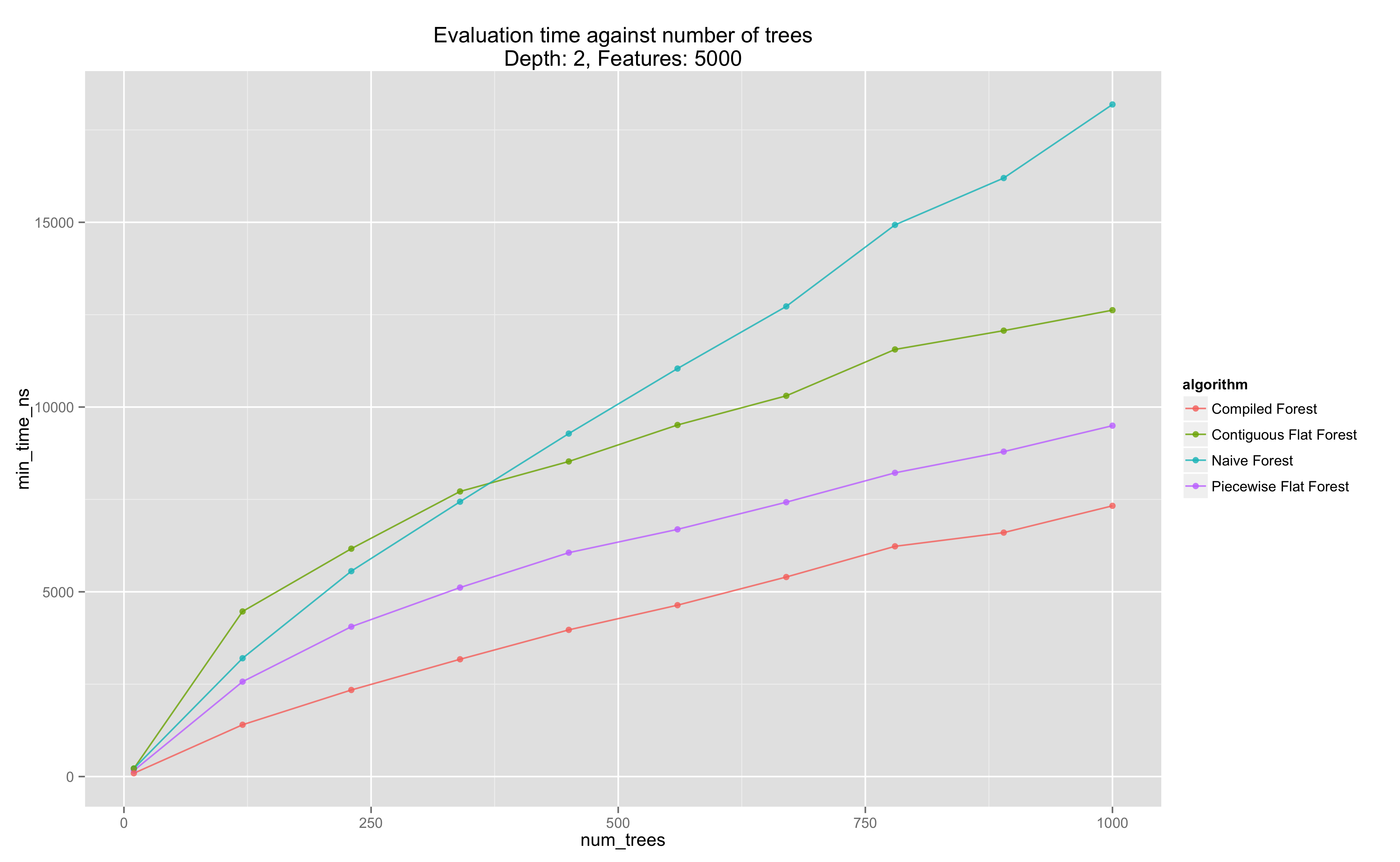
Performance Evaluation

As the student report indicates, the relative performance of each strategy depends on the size of the trees, the number of trees, and the number of features in the given feature vector.

Our methodology is to generate a random ensemble with a given depth, number of trees, and number of features, construct the evaluators of this tree for each strategy, and measure the evaluation time of each strategy across a set of randomly generated feature vectors. (We also check correctness of the implementations via a QuickCheck style test that each strategy computes the same result for a given feature vector).

\begin{align} \text{num_trees} &\in [1, 1000] \\ \text{depth} &\in [1, 6] \\ \text{num_features} &\in [1, 10000] \end{align}

Visualization

We look at trellis plots of the evaluation time against number of trees, for the various evaluation strategies.

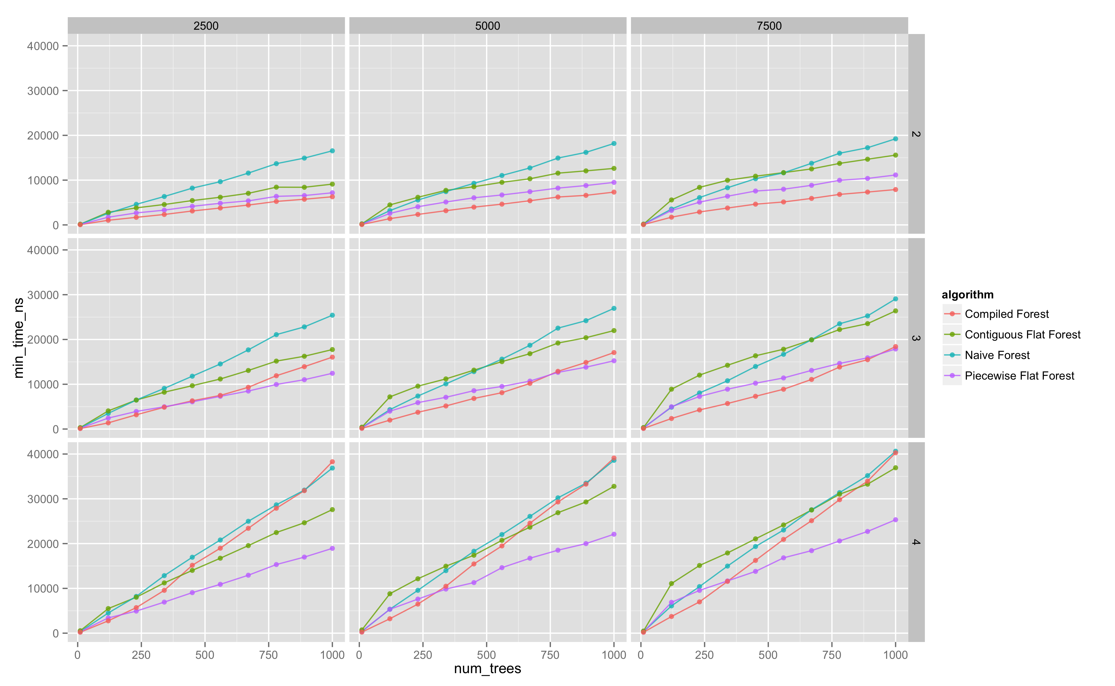
The following diagram is the entire parameter space explored (click for more detail).

Regression

To quantify these effects on the cost of evaluation for the different algorithms, we fit a linear model against these covariates, conditioned on the algorithm used. Conceptually, we are just splitting our dataset by the algorithm used, and fitting a separate linear model on each of these subsets.

(as an aside - the R formula syntax is a great example of a DSL done right.)

We see $R^2$ values ~0.75-0.85 with all coefficients, with almost all coefficients statistically different from zero at the 0.1% level - so we can draw some provisional inferences from this model.

We note:

• the compiled tree strategy is much more sensitive to the depth of the decision tree, which aligns with observations made in the student report.
• the compiled tree strategy and the naive strategy are also more sensitive to the number of trees than the flattened evaluation strategy. Thus for models with huge numbers of trees, the flattened evaluation may be the best.
• The intercept term for the compiled tree is the most negative - thus for 'small' models - low number of trees of small depth, the compiled tree approach may be the best evaluation strategy.

Conclusions

We've implemented and analyzed the performance of a selection of decision tree evaluation strategies. It appears there are two main conclusions:

• For small models - <200 or so trees with average depth <2, the compiled evaluation strategy is the fastest.
• For larger models, the piecewise flattened evaluation strategy is most likely the fastest.
• Choosing the right evaluation strategy can, in the right places, improve performance by greater than 2x.

Next, I'll look at implementing these methods in some commonly used open-source ML packages, such as scikit-learn.